
|
Week Twenty-Two CalTRACK Update Last week marked the final CalTRACK 2.0 working group meeting. In this meeting we discussed an update to hourly methods, an overview of our progress during CalTRACK 2.0, and suggestions for CalTRACK 3.0. You can view the final meeting at following link: Hourly Methods Update: Empirical testing has shown correlation between energy consumption and season in residential buildings, that can have an effect on the savings error. The CalTRACK 2.0 working group has proposed accounting for this seasonal effect by shortening the 12-month baseline period to 3-month weighted baseline periods. The figure below shows the effect of shortening baseline periods to 3-month on Normalized Mean Bias Error (NMBE) for residential buildings. 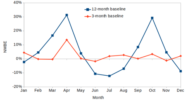 However, shortening an annual baseline to 3-month weighted baselines may not be necessary for all building types. Notably, commercial buildings tend to have a smaller seasonal effect than residential buildings, and may not experience increased NMBE from using a 12-month baseline period. The working group has established the following NMBE thresholds to define buildings that require 3-month weighted baselines and those where an annual baseline period is acceptable.
CalTRACK 2.0 Recap: Since February, the CalTRACK 2.0 process has tackled several major issues. Below is a quick synopsis of the major tasks addressed and outcomes for these topics.  Task 1: Updates to CalTRACK daily and billing methods based on feedback from CalTRACK 1.0 users. Some updates include:
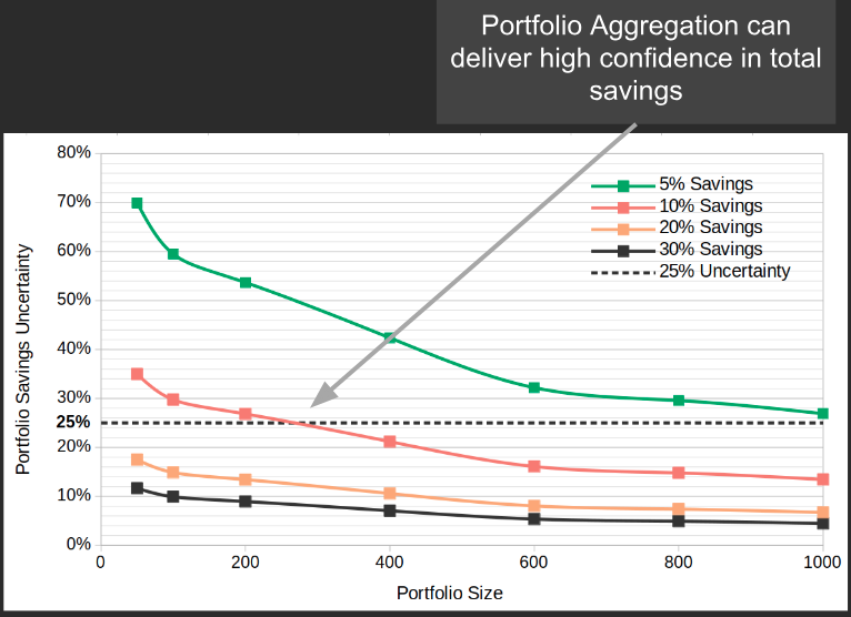 Task 2: Assess the feasibility of a portfolio aggregation approach for calculating savings as well as any effects on savings uncertainty.
Task 3: Develop a prototype method for calculating hourly savings.
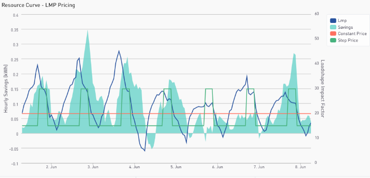
Task 4: Demonstrate how price signals can adjust the value of hourly load shapes to match procurement needs.
 CalTRACK 3.0: The direction of CalTRACK 2.0 methods development was guided by feedback from use cases that required “payable savings”. For example, PG&E’s pay-for-performance energy efficiency program decided to increase compensation for energy savings during peak hours during the second iteration of their program. This required CalTRACK 2.0 to develop methods that generate savings estimates at the hourly level. Similarly, we expect CalTRACK 3.0’s tasks will be guided by the demands of stakeholders that implement programs using CalTRACK 2.0 methods. In addition, we have designed a CalTRACK 3.0 sandbox on GitHub to document issues that require further investigation. We encourage working group members to continue adding ideas to the CalTRACK 3.0 sandbox as they arise. Homework:
0 Comments
Week Twenty One CalTRACK Update  Energy efficiency and other distributed energy resources have the potential to bring value to the grid. The value of energy efficiency in particular has been calculated with averaged assumptions about avoided costs of producing, procuring and distributing energy from fossil fuel infrastructure, as well as other factors in some cases (e.g. avoided emissions, societal benefits etc.). This valuation is estimated at the regulatory level, when assessing the cost-effectiveness of energy efficiency, but it is usually sequestered from market actors, who have the most control over actual generated energy savings. While pay-for-performance is a key step to aligning the value of energy efficiency with the market actors responsible for it, using total annual savings as the performance metric conceals the time- and location-based value of energy efficiency which can vary significantly. This current disconnect of energy efficiency savings to its actual value to the grid or emissions avoided is an area ripe for improvements in modeling and understanding the real value of delivered energy savings. Furthermore, it is critical if energy efficiency wants to have a place at the integrated resource planning table. The availability of both hourly savings AND hourly valuations for those savings (e.g. avoided costs or emissions) allows program administrators to estimate, to a much better degree of accuracy, the value of energy efficiency to the grid. In last week’s working group discussion we covered the topic of valuation in the context of hourly load shape analysis conducted through CalTRACK 2.0. Introduction Portfolio load shapes can be used by programs that compensate for hourly energy savings and whose intention is to align the incentives with savings that are valuable to the grid when it is needed. The construction of portfolio load shapes requires:
To calculate hourly energy savings, CalTRACK methods utilize a time-of-week and temperature model. To value the energy savings, a valuation method must be applied to the hourly savings calculations. Overview of Valuation Methods There are a range of valuation strategies one can consider; which may have different effects on the outcomes. 1. Constant Valuation Energy savings are valued at a constant price across all hours of the year. 2. Step Valuation During Peak Energy savings are valued higher during peak hours of day. This valuation method assumes the peak period is the same across all days. For example, a step valuation may value energy savings from 5-8 PM 3 times more than non-peak hours of the day. 3. Avoided Cost Valuation Energy savings are valued based on their hourly avoided costs, which provides a unique value for each hour of the year. The total avoided costs include costs associated with transmission, distribution, resource portfolios, carbon and more. 4. Avoided Energy Valuation Energy savings are valued based on the cost of generating a unit of energy at the given time and location. This is similar to Avoided Cost Valuation, but only costs of generating energy are considered. Overview of Examined Scenarios Different programs and even different measures within a program will deliver different types of time-based value even if their annual savings seem similar. Here are three fairly common cases to consider for this example: 1. Home Performance Scenario Home performance improvements, which are primarily focused on weatherization and HVAC, have concentrated energy savings during periods of high and low temperatures, with little to no savings in the shoulder seasons. For example, insulated windows will generate energy savings from reduced heating during the winter and air conditioning during the summer. 2. Lighting Scenario Lighting improvements provide consistent savings year round, during hours when lighting is required. 3. Load Shifting Scenario Load shifting equipment moves energy load from high demand periods to lower demand periods. An example is an air conditioning demand response program that reduces electricity demand during peak hours. Net energy savings from load shifting programs are typically low or neutral because they cause increased energy consumption before and after the high demand period. Scenario Load Shape Analysis In the table below, the home performance, lighting, and load shifting scenarios were compared with different valuation methods. The numbers in this table represent relative value across programs (i.e. they are unit-less), making the comparison of the different methods for a particular measure/program not very meaningful. However, when each row in the table is examined separately, the type of savings that are encouraged by each valuation scheme becomes apparent. 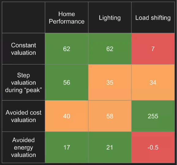 The valuation scheme will usually be a policy, market or procurement decision that should consider the ultimate outcomes intended - to ensure incentives and motivation can be aligned.
For example, if a program aims to reduce electricity grid operating costs, then an avoided cost is the most appropriate valuation method. Under this valuation method, the load shifting program is most effective. However, if a program aims to reduce net energy use, avoided energy valuation may be the most appropriate method. In this context, a market actor may decide that a lighting program is their best option. |
The purpose of this blog is to provide a high-level overview of CalTrack progress.
For a deeper understanding or to provide input on technical aspects of CalTrack, refer to the GitHub issues page (https://github.com/CalTRACK-2/caltrack/issues). Recordings
2019 CalTRACK Kick Off:
CalTRACK 2.0 July 19, 2018 June 28, 2018 June 7, 2018 May 24, 2018 May 3, 2018 April 12, 2018 March 29, 2018 March 15, 2018 March 1, 2018 February 15, 2018 February 1, 2018 Archives
March 2024
|
 RSS Feed
