
|
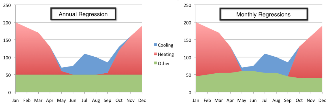
Week Twenty CalTRACK Update Over the past three weeks, CalTRACK methods testing has revolved around issues that need resolution to facilitate pay-for-performance using hourly savings. In particular, the focus has been on (i) testing and validating the Time-Of-Week and Temperature model for residential buildings and (ii) scenario analysis of different valuation methods for hourly savings. Other working group members (particularly Home Energy Analytics) contributed significant empirical results that will help in improving the robustness of the CalTRACK methods. This type of participation is the foundation for improving CalTRACK methods. Thank you for the great work! Hourly methods improvements Background: The default Time-Of-Week and Temperature model allows for extended baseline periods when fitting baseline models. When the model adaptation function is not used, a single model can be fit to the entire baseline period, which could be up to 12 months long. The single, yearly regression approach assumes that base load and weather sensitivity of energy consumption is constant throughout the year. Empirical Results: Empirical evidence shows that baseline and weather-related energy use varies during different months of the year. This variation is not represented when a single regression is estimated for the entire baseline period. Below are two potential modeling approaches:
 One potential problem that appears when models are fit with data from limited time periods is that without many data points, they tend to overfit the data. We can see evidence of overfitting by looking at the relationship of model error from within-sample to the model error when applied to out-of-sample data. Large discrepancies between the two values indicate potential overfitting. This relationship is evident in the figure below. 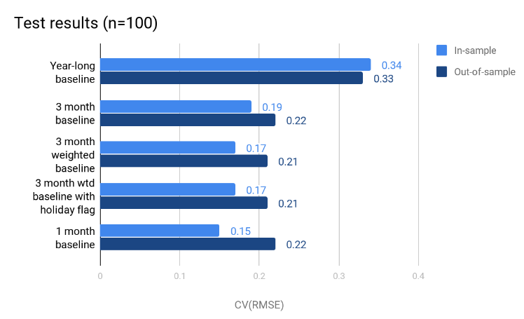 Recommendation:
After reviewing the results of the empirical testing, we recommend applying a three-month weighted regression model for residential hourly methods. Twelve models will be fit for each month of the year, with months before and after the month of interest weighted down by 50%. For example, when predicting the counterfactual energy usage for the month of July, the corresponding baseline model will be fit using data from June, July and August of the previous year. The data points from June and August will be assigned a 50% weight compared to the data points from July. This approach accounts for varying energy consumption patterns across months of the reporting period without overfitting the model to limited data. Keep an eye out for next week’s blog post where we’ll summarize the testing of valuation methods for hourly savings.
6 Comments
Week Eighteen CalTRACK Update Our second week of discussion on hourly portfolios included a working group meeting. You can watch the full meeting here: The value of hourly energy savings varies by use case. As such, the CalTRACK framework should be flexible to accomodate for the priorities of different use cases. A load impact factor assigns more value to energy savings during certain hours of the reporting period. For example, if a utility values energy savings 3 times more from 4-8 PM, then hourly energy savings will be multiplied by a load impact factor of three during the hours of 4-8 PM for each day of the reporting period. Each use case may need to define the load impact factors according to their desired outcomes. The portfolio-level savings are calculated by multiplying estimated hourly energy savings by the hourly load impact factor and aggregating across all hours in the reporting period. In the working group meeting we reviewed three basic methods calculating portfolio-level energy demand savings: Constant Marginal Pricing: A constant marginal pricing scheme uniformly values energy savings at each hour of the year. In this case, the load impact factor for each hour of the year is 1. This method is the simplest to compute and does not require additional data, but it fails to account for load impacts of energy savings. Static Peak Pricing: A static peak pricing scheme accounts for increased value of energy savings during peak consumption periods. A certain range of hours (ie-4-8 PM) is defined as the daily peak consumption period. The designated peak consumption period is imposed on all days of the reporting period. Static peak pricing assigns hourly load impact factors of 1 to all hours except for hours during the peak consumption period. Peak consumption period hours are given load impact factors that are greater than 1, which reflects the higher value of energy savings during these hours. Although Static Peak Pricing accounts for load impacts, its price signals are imperfect because they assume a constant peak consumption period. In reality, the peak consumption period varies throughout days of the year due to seasonality and other energy consumption trends. Real-Time Pricing: A Real-Time Pricing scheme assigns a unique load impact multiplier to each hour of the year. The load impact multipliers can be calculated according to locational marginal energy prices (LMPs). The real-time pricing scheme provides the most accurate price signals for energy savings with respect to grid impacts. The Real-Time Pricing scheme generates the most accurate price signals, but requires LMP data and there is uncertainty in hourly prices. 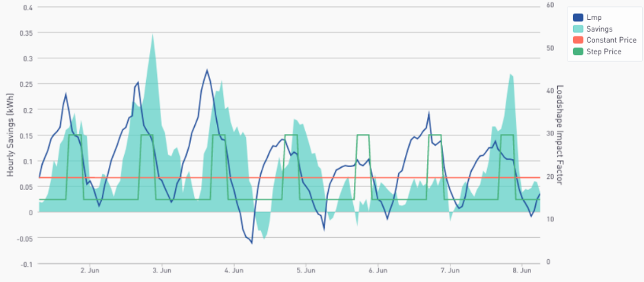 Empirical Testing:
In the coming weeks, we would like to empirically test methods for calculating portfolio-level energy savings for common use cases. Some use cases include:
Week Seventeen CalTRACK Update Establishing guidelines for aggregating building-level hourly energy savings into portfolio loadshapes requires careful consideration of information and uncertainty-level preferences for various use cases. The issues with aggregating energy savings for hourly methods and potential solutions are outlined below:  Aggregation Method for Billing Period and Daily Methods: In daily and billing period methods, building-level savings are generated by summing the building’s estimated energy savings for each day or billing period of the reporting period. The portfolio savings are then calculated by aggregating total savings for each building in the portfolio. Why are daily and billing period aggregation methods problematic with hourly models? For hourly models, portfolio uncertainty is difficult to calculate when savings are aggregated for each hour due to correlation in the error term. Suggested Hourly Aggregation Methods: To begin our discussion of hourly aggregation methods, consider two types of roll-ups: Vertical Roll-Ups: In a vertical roll-up, hours within a day are grouped together for each building before aggregation. For example, one may choose to aggregate hourly energy savings in three-hour intervals throughout the day instead of each hour individually. Although vertical roll-ups can reduce portfolio uncertainty, larger time intervals provide less information in portfolio loadshapes. Hourly methods are created to provide granular information about energy load impacts during each time-of-day. Less information is available if hours are “rolled-up” into larger time intervals. Horizontal Roll-Ups: Horizontal roll-ups aggregate each hourly estimate with estimates of the same hour across weeks. A horizontal roll-up can aggregate individual hours or time intervals, such as the three-hour interval discussed above.  Other Considerations: There were a few additional suggestions from the working meeting (5/24) that could help create guidelines for aggregating portfolio loadshapes:
Homework:
|
The purpose of this blog is to provide a high-level overview of CalTrack progress.
For a deeper understanding or to provide input on technical aspects of CalTrack, refer to the GitHub issues page (https://github.com/CalTRACK-2/caltrack/issues). Recordings
2019 CalTRACK Kick Off:
CalTRACK 2.0 July 19, 2018 June 28, 2018 June 7, 2018 May 24, 2018 May 3, 2018 April 12, 2018 March 29, 2018 March 15, 2018 March 1, 2018 February 15, 2018 February 1, 2018 Archives
March 2024
|
 RSS Feed
