Tackling Hourly Savings for a Portfolio

Week Eighteen CalTRACK Update

Our second week of discussion on hourly portfolios included a working group meeting.  You can watch the full meeting here: ​

June 7, 2018 Working Group Meeting Link

The value of hourly energy savings varies by use case. As such, the CalTRACK framework should be flexible to accomodate for the priorities of different use cases. A load impact factor assigns more value to energy savings during certain hours of the reporting period. For example, if a utility values energy savings 3 times more from 4-8 PM, then hourly energy savings will be multiplied by a load impact factor of three during the hours of 4-8 PM for each day of the reporting period. Each use case may need to define the load impact factors according to their desired outcomes.

​The portfolio-level savings are calculated by multiplying estimated hourly energy savings by the hourly load impact factor and aggregating across all hours in the reporting period. In the working group meeting we reviewed three basic methods calculating portfolio-level energy demand savings:

Constant Marginal Pricing:
A constant marginal pricing scheme uniformly values energy savings at each hour of the year. In this case, the load impact factor for each hour of the year is 1. This method is the simplest to compute and does not require additional data, but it fails to account for load impacts of energy savings.

Static Peak Pricing:
A static peak pricing scheme accounts for increased value of energy savings during peak consumption periods. A certain range of hours (ie-4-8 PM) is defined as the daily peak consumption period. The designated peak consumption period is imposed on all days of the reporting period. Static peak pricing assigns hourly load impact factors of 1 to all hours except for hours during the peak consumption period. Peak consumption period hours are given load impact factors that are greater than 1, which reflects the higher value of energy savings during these hours. Although Static Peak Pricing accounts for load impacts, its price signals are imperfect because they assume a constant peak consumption period. In reality, the peak consumption period varies throughout days of the year due to seasonality and other energy consumption trends.

​Real-Time Pricing:
A Real-Time Pricing scheme assigns a unique load impact multiplier to each hour of the year. The load impact multipliers can be calculated according to locational marginal energy prices (LMPs). The real-time pricing scheme provides the most accurate price signals for energy savings with respect to grid impacts. The Real-Time Pricing scheme generates the most accurate price signals, but requires LMP data and there is uncertainty in hourly prices.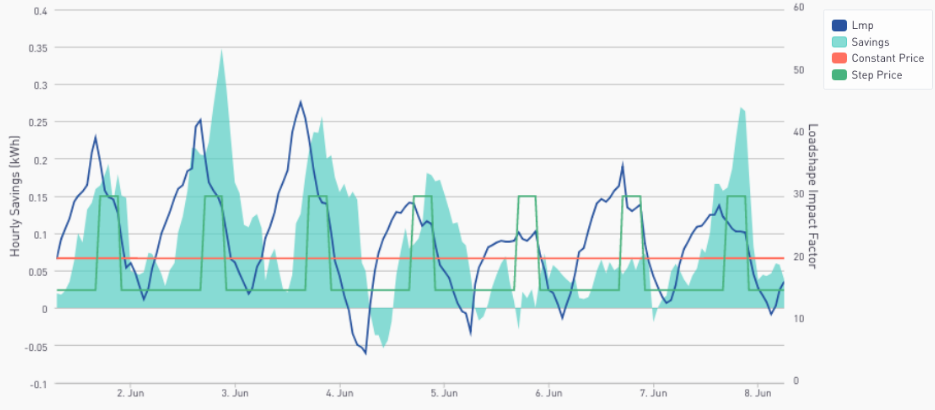

Empirical Testing:
In the coming weeks, we would like to empirically test methods for calculating portfolio-level energy savings for common use cases. Some use cases include:

1. Programs that reduce kWh consumption without considering load shifting
   
2. Load shifting programs that reduce kW
   

Homework:

1. Review final methods documentation and provide comments on pull request on GitHub
2. Review final hourly methods on GitHub
3. Provide feedback on load shape results on GitHub
4. ​Contribute to the Sand Box of future issues