Results from Daily & Billing Period Methods Testing

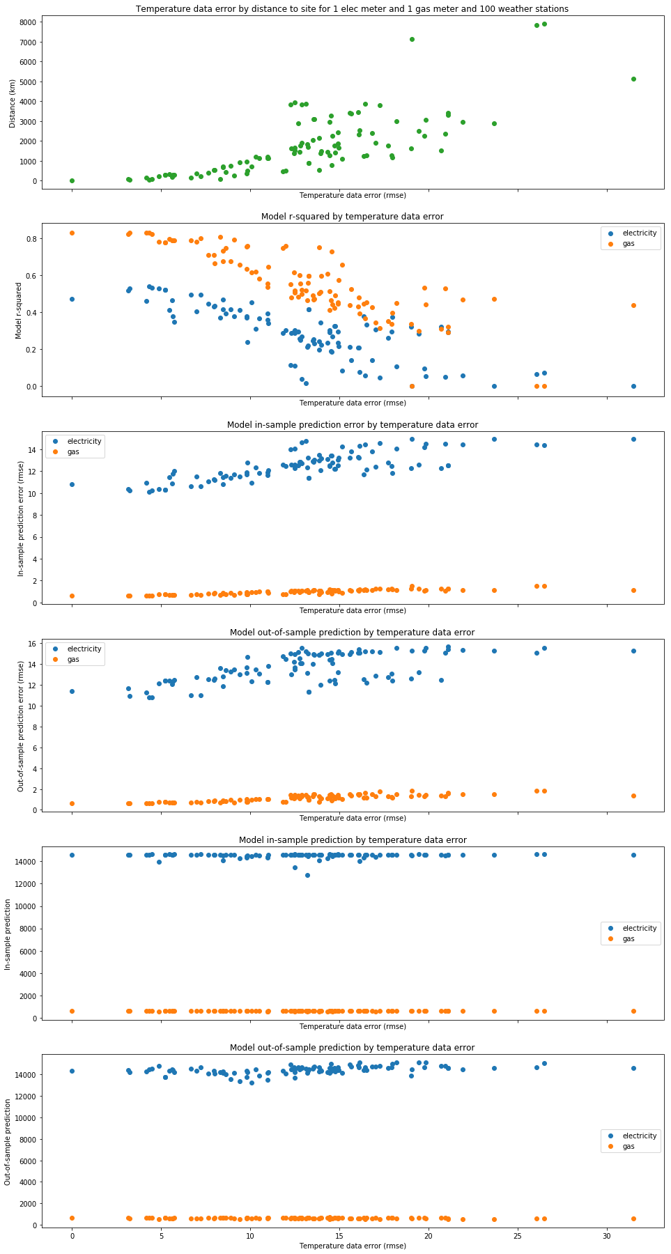
Week Four CalTRACK Update

During week 4, we received some interesting results from tests on daily and billing period methods. In this week’s blog post, we analyze the test results and determine their effect on our proposed daily and billing period methods. Additionally, we will introduce the new topic of building qualifications. ​
(Participant Homework can be found at the bottom of this post)

​Test Results:

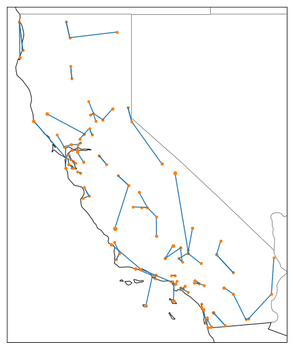
Weather Station Mapping: 
Because we do not have access to weather data at the location of each site, the best approach for estimating a site’s temperature is to use data from nearby, high-quality weather stations. The most intuitive way to “map” which primary and backup weather stations to use for a site is to simply choose weather stations with the shortest distance to the site. Some argue that this simple method fails to account for the unequal distribution of weather patterns over space. For example, imagine a mountain home is technically closer to a weather station in the desert valley than to another weather station in the mountains. We might expect the house’s weather data to be better approximated by the mountain weather station than the desert valley weather station, despite it being further away. To account for this phenomenon, another proposal is to use pre-defined climate zones throughout states to choose the closest primary and backup weather stations that are within that site’s climate zone.

Two proposals for mapping a site’s  weather stations:

• Method 1: Choosing the primary and backup weather stations that are closest to the site
• Method 2: Choosing the primary and backup weather stations that are closest to the site and within the same climate zone

To empirically inform our decision, we ran a simulation for each mapping method where we used the actual weather stations as units, instead of the sites, and compared each method’s accuracy. Our results show that both proposed methods provide very similar results, with “Method 1” and “Method 2” providing a perfect match 53% and 56% of total matches respectively. These results indicate that there are not significant accuracy reductions from choosing the simpler “Method 1".

---

---

The Importance of Exact Weather Data:

The purpose of our weather station mapping methods are to ensure that each site has the best possible estimation of their “true” weather values. Because there is uncertainty in estimation of each site’s weather values, a question that follows is: “how important is the accuracy of weather data when predicting energy savings?” To answer this question, we did an empirical experiment that provides some insight.

The Experiment:

• We took data from 1 electricity meter and 1 gas meter
• We ran a model using data from climate zone weather station mapping (Method 2)
• With the same meter data, we ran the same model but used weather data from a set of 2 weather stations for all 50 states in the USA. There is significant weather diversity in the USA, so these results indicate the effect of inaccurate weather on model prediction.
• We analyzed the results. In the graphs, there is a dot for each model. This includes a dot for each of the 50 states and one dot for climate zone mapping. ​​

CLICK TO ENLARGE

Results: 

• Although there are some moderate increases in data error and reduction in model fit that result from adding very inaccurate weather data, our results show that the predicted energy savings are remarkably robust to changes in weather data. This indicates that the accuracy of weather data does not have a significant effect on annual energy savings predictions, even in extreme cases.
• It would be very useful to see this hypothesis tested with more data

---

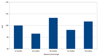
Maximum Baseline Period Length:
There have been discussions about defining a maximum baseline period because excessively long baseline periods may absorb unnecessary variation that could obscure our model predictions. To determine the effect of longer baseline periods, we calculated baselines of 12, 15, 18, 21, and 24 months. The graph below shows that normalized annual consumption (NAC) can be unstable as we increase the baseline period.
​
Recommendation:

• We recommend using a 12 month baseline as it is most indicative of the period immediately prior to the intervention.
• It would be reassuring to see these findings confirmed by others in different datasets

---

---

Degree Day Balance Points:
A proposed new method for CalTRACK 2.0 is to use variable balance points instead of fixed balance points on the HDD and CDD variables. In the figure below, we can see that buildings tend to cluster at the limits of balance point degree ranges, which implies that some results may be constrained by small search grids. When the degree range is expanded, the results displays a distribution that is closer to Gaussian.

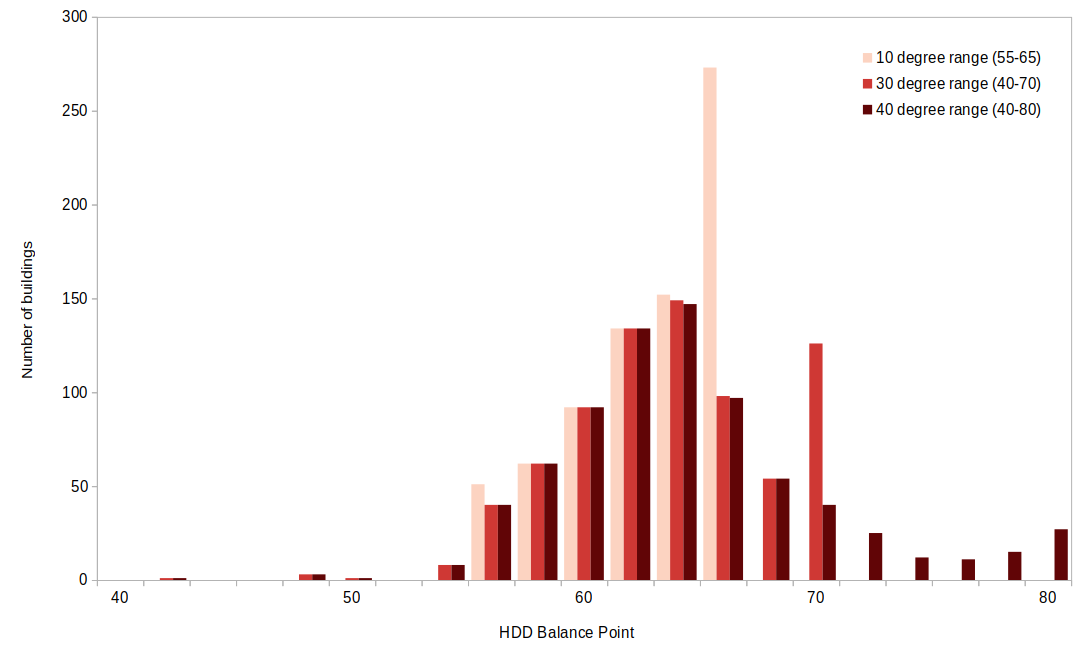
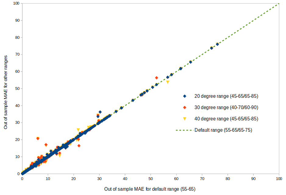
Although expanding the search grid may uncover a balance point that yields a higher R-squared, the figure on the right shows that these results have a nominal impact on model fit. Regardless, variable balance points are advised because they provide better balance point estimates, which have more interpretation value.
​
​Recommended Allowable Ranges:
HDD: 40-80
CDD: 50-90

---

---

Model Selection Criteria
In CalTRACK 1.0, model selection criteria involved:

1. Filtering out estimators with insignificant p-values (greater than 0.1) and
2. Choosing model based on the adjusted R squared​

In CalTRACK 2.0, we intend to eliminate the p-value screen and select models strictly on the adjusted R squared. We suggest this change because the p-value screen does not increase our model fit and we lose valuable information on estimators when we drop them due to high p-values, as well as eliminating many weather-sensitive model fits.

---

Handling Billing Data:
Modeling using billing data was underspecified in CalTRACK 1.0. We are proposing to include explicit instructions on modeling using billing data that includes billing periods of different lengths using weighted least squares regression.

---

​New Topics:

Building Qualification:
In this coming week, we will begin our examination of building qualification screening criteria. The CalTRACK methods were initially tested using residential buildings and are currently mainly used to quantify energy savings for residential units and small commercial buildings. The limits of the CalTRACK methods for measuring savings in commercial or industrial buildings (where weather is likely to be a poorer predictor of energy consumption) has been subject to less scrutiny. Our goal is to create empirical tests for determining the energy usage patterns in buildings that qualify a building for CalTRACK methods and exclude those that would be better estimated with different methods. We are looking forward to your input on potential methods and tests to define buildings that qualify for CalTRACK.

Some questions that need to be addressed (and we welcome additional questions):

• When should we accept intercept only (non-weather based) models? What's a good metric to assess an intercept-only model fit?
• How do our metrics and methods align with pay-for-performance programs? Do they reflect performance risk and uncertainty? Are they convenient for implementers and aggregators?
• What should we do with disqualified buildings? Are they eliminated from participating in pay-for-performance programs or is there another way to accommodate them?
• What metrics and thresholds are useful for assessing baseline model fit in a pay-for-performance context?​

We are looking forward to your input on building qualification in this coming week. There will be a lot to discuss on GitHub Issues. We would like to test proposed building qualification methods empirically before making decisions, so it is important to make method and testing suggestions as soon as possible.

---

HOMEWORK:

1. This is the last chance to make suggestions on proposed updates to daily and billing period methods in "FINAL CALL FOR COMMENTS: Monthly and Daily Methods Updates"
   • Post comments or alternative results on GitHub before the issue closes
   • If you have a comment on the final specifications after the issue is closed, address this in a new issue
2. Post questions, comments, research, or testing ideas on Building Qualifications in GitHub Issues.