Hourly Methods for Pay for Performance

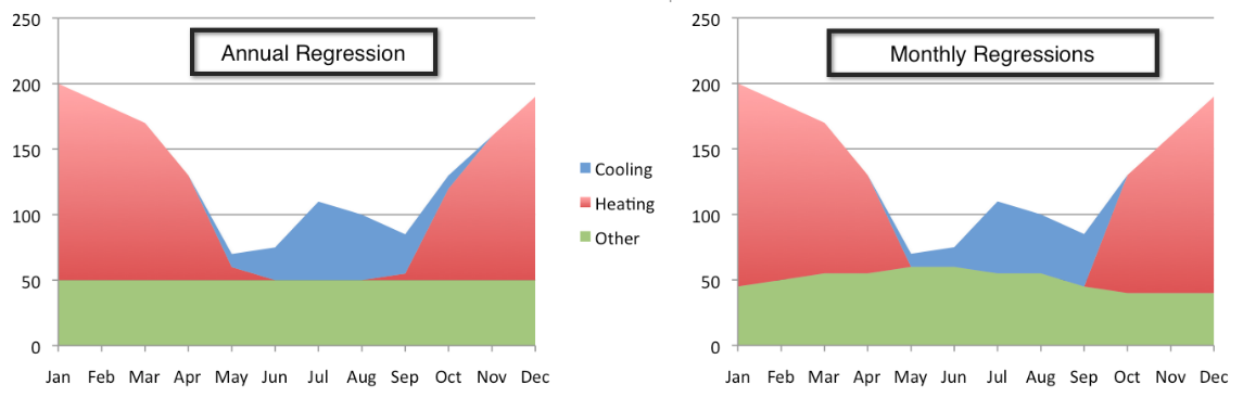
Week Twenty CalTRACK Update

Over the past three weeks, CalTRACK methods testing has revolved around issues that need resolution to facilitate pay-for-performance using hourly savings. In particular, the focus has been on (i) testing and validating the Time-Of-Week and Temperature model for residential buildings and (ii) scenario analysis of different valuation methods for hourly savings. Other working group members (particularly Home Energy Analytics) contributed significant empirical results that will help in improving the robustness of the CalTRACK methods. This type of participation is the foundation for improving CalTRACK methods. Thank you for the great work!

June 28, 2018 Working Group Recording

Hourly methods improvements
Background:
The default Time-Of-Week and Temperature model allows for extended baseline periods when fitting baseline models. When the model adaptation function is not used, a single model can be fit to the entire baseline period, which could be up to 12 months long.  The single, yearly regression approach assumes that base load and weather sensitivity of energy consumption is constant throughout the year.

Empirical Results: 
Empirical evidence shows that baseline and weather-related energy use varies during different months of the year. This variation is not represented when a single regression is estimated for the entire baseline period. Below are two potential modeling approaches:

1. A regression approach that estimates one model for the entire baseline period, which is 1 year in this case.
   
2. A regression approach that estimates 12 models for each month of the baseline period, which is 1 year in this case.
   

It is evident that base load energy consumption, which is the green portion of the graphs below, is not constant throughout the year. The failure to account for varying base load energy consumption across the baseline period contributes to higher model variance, measured by CVRMSE, in CalTRACK methods.

One potential problem that appears when models are fit with data from limited time periods is that without many data points, they tend to overfit the data. We can see evidence of overfitting by looking at the relationship of model error from within-sample to the model error when applied to out-of-sample data. Large discrepancies between the two values indicate potential overfitting. This relationship is evident in the figure below. ​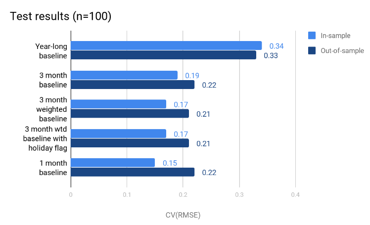

Recommendation:
After reviewing the results of the empirical testing, we recommend applying a three-month weighted regression model for residential hourly methods. Twelve models will be fit for each month of the year, with months before and after the month of interest weighted down by 50%. For example, when predicting the counterfactual energy usage for the month of July, the corresponding baseline model will be fit using data from June, July and August of the previous year. The data points from June and August will be assigned a 50% weight compared to the data points from July. This approach accounts for varying energy consumption patterns across months of the reporting period without overfitting the model to limited data.
​
Keep an eye out for next week’s blog post where we’ll summarize the testing of valuation methods for hourly savings.

Homework:

• Review final methods documentation and provide comments on pull request on GitHub
  
• Review final hourly methods on GitHub
  
• Provide feedback on portfolio load shape results on GitHub
  
• Contribute to the Sand Box of future issues
  

The next working group meeting is in 3 weeks on July 19, 2018.