
|
Thanks to everyone who joined for this month's OpenEEmeter working group. We're excited at the huge progress we're making on CalTRACK 2.1, and greatly appreciate all who have taken time out of their schedule to participate in this important discussion.
Tim Guiterman from Sealed led off yesterday's discussion with a follow-up conversation on revising CalTRACK's requirements to permit its usage with delivered fuels such as propane and heating oil. Because these fuels are delivered and manually refilled, data for them are not as consistent nor as abundant as metered energy is. Tim and the Sealed team proposed making an exception to the 70 day data limit for delivered fuels. The group discussed what the minimum number of data points should be and various factors that could alter this. There was also discussion of relaxing the 365 day baseline period to allow for more data when fitting this period. Most delivered fuel customers can provide data in the form of bills that cover years of time. Adam pointed out that while there might not be a perfect answer to the delivered fuel problem, using the CalTRACK approach is still much better than deemed approaches which are much less accurate. The conversation concluded with Tim agreeing to analyze Sealed data so that the working group can make a data-driven decision on if rule changes should be made for delivered fuel customers and if so what should the minimum requirements be, with proof that backs up these revisions. Adam and Travis then summarized CalTRACK 2.0's deficiencies and how the nearly final model of CalTRACK 2.1 rectifies them. The main problem the team was attempting to solve was seasonal bias in the CalTRACK 2.0 model found primarily in gas meters. They showed that CalTRACK 2.1 has significantly reduced seasonal bias. At the same time it has been necessary to revisit how fast the model can be fit in. Travis has implemented several clever means of speeding up the model from worst-case scenarios of 1 minute to fit down to 10 seconds. He also went into detail about how CalTRACK 2.1 differs from CalTRACK 2.0 in order to solve the issues laid out prior. Additionally, Travis briefly mentions that they have implemented a CalTRACK 2.0 mode, a legacy mode, which can replicate CalTRACK 2.0 results with all of the speed improvements developed recently. Overall, they show that CalTRACK 2.1 reduces seasonal bias by 74% and is between 2 and 100 times faster than CalTRACK 2.0, depending on how it's used (legacy mode or not). Adam and Travis anticipate that by the next meeting, the final CalTRACK 2.1 model will have completed its R&D phase. Next steps involve code cleanup, polishing, and documentation so that CalTRACK 2.1 can be integrated into the OpenEEmeter. Next Meeting Scheduled: Tuesday, June 6th, 1pm PT. Watch the full presentation below.
0 Comments
Thanks to everyone who joined the most recent OpenEEmeter working group meeting.
Tim Guiterman from Sealed led off the conversation with a discussion of the need to address delivered fuels such as propane or heating oil in the CalTRACK specifications. CalTRACK's current data sufficiency requirements often limit the ability to model homes that using delivered fuels, which are common in the Northeast. Because these fuels are not necessarily delivered on a consistent cadence, CalTRACK's monthly data requirements are barrier to using it for these kinds of customers. Making CalTRACK more accessible and avoiding unnecessary disqualifications is particularly important given the new funding from the IRA and the opportunities it presents for adopting a measured pathway for incentives. Adam Sheer and Travis Sikes then shared updates and results related to the CalTRACK Daily 2.1 model, which is nearing completion. Adam reviewed the issues CalTRACK 2.1 process is attempting to address around model bias, and the tradeoffs between adding parameters to correct bias and the need to avoid overfitting. Preliminary results on the new 2.1 model showed a dramatic improvement, reducing summer, winter and weekend bias. Getting these kinds of improvements requires additional computations. CalTRACK 2.0 performance prohibits any additional complexity due to the time it takes to fit a model (20 - 60 seconds). This is particularly prohibitive to the cross-validation that is the lynchpin of our current improvement efforts. To address this, Travis gave an extended presentation of how he has dramatically improved the computational efficiency of the OpenEEmeter, reducing the per-meter fitting time from 20 to 60 seconds to approximately 0.5 seconds (20-120 times faster) for an equivalent fit. For those that need or want to run the original CalTRACK 2.0, a CalTRACK 2.0 legacy mode will be included that has all of these computational efficiency improvements. The team discussed the remaining steps needed to finalize the model formulation and are hopeful that it will be wrapped up in the next one to two months. We are excited about the progress made so far and the potential impact of the updated model. Watch the full meeting below. Next Meeting Scheduled: Tuesday, May 2nd, 1pm PT
Thanks to everyone who joined us for yesterday's OpenEEMeter technical working group meeting.
Adam Scheer led off the meeting by reiterating the high-level goals for the CalTRACK 2.1 Daily model which are to improve specific and known areas of model bias and gain computational efficiency in the process. He explained the need to solve seasonal and weekend/weekday bias by adding parameters and optimization steps without creating an overfitting problem or making the model so complex that it can't be scaled to hundreds of thousands or millions of meters. For the CalTRACK Hourly model, Adam laid out issues to discuss in future meetings, including remedying known small bugs, specifying demand response baselines, and incorporating solar PV modeling. Adam then introduced James Fenna from Carbon Co-op to discuss some challenges and modifications needed to implement CalTRACK (specifically eeweather) in the U.K. and internationally. In particular, James discussed the problems of calibrating for metric temperatures and the need for different sources of weather data internationally. Adam then led a more detailed discussion of the specific tradeoffs of adding parameters to address seasonal bias in the model. The group discussed how seasonal bias is a problem that has been known for decades, and how much effort should be put into improving the Daily model versus Hourly. Watch the full meeting below. Next Meeting Scheduled: Tuesday, April 4th, 10am ET, 1pm PT Join the working group to get access by clicking this link:
Download the presentation slides below
Thanks to all who attended the most recent CalTRACK working group meeting.
McGee Young opened this meeting with some words for Shuli Goodman of LFEnergy Foundation who recently passed away. McGee made the point that Shuli was instrumental in helping to give the OpenEEmeter credibility and a home. Shuli had a vision that open source/open standards could do for energy what it's done for other industries, like the Internet. Under her leadership LFEnergy has grown as an umbrella to many innovative projects. She will be missed. The technical discussion explained the current goal of examining sources of bias or error in CalTRACK 2.0 and potential solutions. The group discussed the need to balance adding additional parameters against the risk of overfitting. Watch the full meeting below. Next Meeting Scheduled: Tuesday, March 7th, 10am ET, 1pm PT Join the working group to get access by clicking this link: 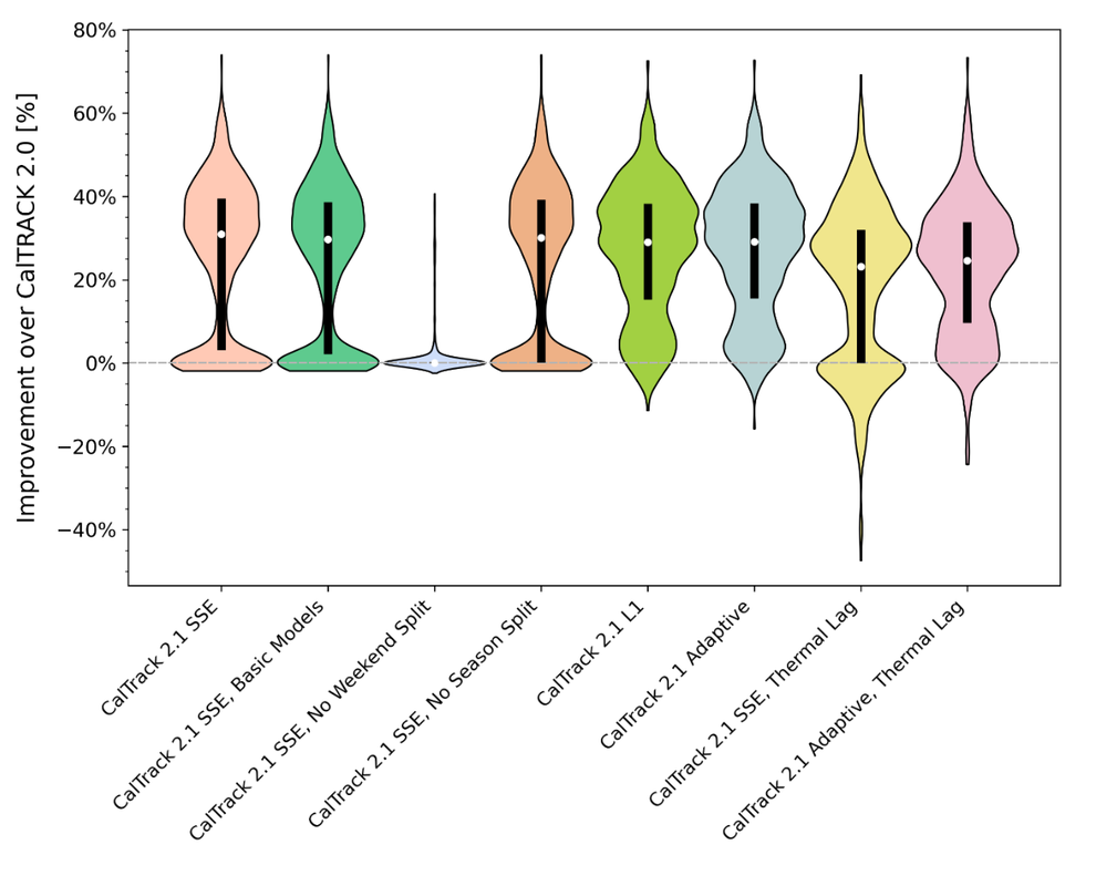 Join the CalTRACK working group to help improve the CalTRACK methods and the LFE OpenEEmeter open-source software. This working group is comprised of many of the leading users of these methods and code. Come join the process! Meeting topics will include
Next Meeting Scheduled: Tuesday the 7th, 10am ET, 1pm PT Join the working group to get access by clicking this link:
Watch the 01/17/2023 technical working group meeting on demand or below. If you haven't signed up yet, click here to register for the next meeting.
Watch the 12/06/2022 technical working group meeting on demand or below. If you haven't signed up yet, click here to register for the next meeting.
Thank you to everyone who was able to make it to our CalTRACK 2.1 | OpenEEmeter kick off on 11/22. If you were unable to attend check out the recording available on demand or below. We look forward to continuing this work at next week's meeting on Tuesday, 12/6/2022.
What Is CalTRACK
The CalTRACK methods and OpenEEmeter codebase are a standard and transparent set of procedures designed to calculate savings based on metered energy consumption. Since their development these procedures have been used to measure the impacts of dozens of energy efficiency programs across the United States and as a settlement tool for performance-based demand flexibility markets. The original CalTRACK working group members included the California Energy Commission, the California Public Utilities Commission, Pacific Gas and Electric Company, DNV GL, Energy Savvy, and a host of other contributing members (CalTRACK history). The OpenEEmeter codebase was donated to Linux Foundation Energy (LFE) as an open-source project in 2019 to culminate the group's efforts. What's Next In the last few years, the need for accurate and standardized meter-based methods has grown, along with the market for scalable and integrated demand-side programs. In 2020-2021, COVID-19 disruptions heightened the importance of identifying and removing the impacts of external (non-program) factors on energy consumption. In partnership with the Department of Energy, Recurve developed the GRIDmeter comparison group methods to address this challenge. Similarly, California's 2020 heat wave and rolling power outages exposed the necessity for more reliable demand response methods. In response, Recurve developed the FLEXmeter methods on behalf of the California Independent System Operator. CalTRACK and GRIDmeter are the foundations of FLEXmeter, which can accurately measure the impact of demand response events, even during extreme heat waves, and, importantly, support integrated EE and DR measurements. While CalTRACK 2.0 is foundational to all of these approaches, we believe that further updates to the methods and the OpenEEmeter code will promote greater accuracy and confidence in the impacts of behind-the-meter resources and could help bring a wider variety of demand-side programs to the table. We look forward to working with other stakeholders and partners who have used CalTRACK and the OpenEEmeter for their own initiatives and would like to contribute to this process. On November 22, 2022 Recurve will host the CalTRACK 2.1 kickoff meeting. The CalTRACK 2.1-OpenEEmeter development process will follow the LFE Charter and Code of Conduct. Methods development is an experimental process that can benefit from the input and experiences of many. The collaborative feedback loop is an exciting aspect of open-source development. The successes and failures at every stage represent progress for all to see and provide many points for collaboration and for new ideas to emerge. We can't wait to get the band back together.  Phil Ngo, Director of Engineering at Recurve, provides insights into the OpenEEmeter and EEweather, which is an open source implementation of the CalTRACK Methods that resides in LF Energy. |
The purpose of this blog is to provide a high-level overview of CalTrack progress.
For a deeper understanding or to provide input on technical aspects of CalTrack, refer to the GitHub issues page (https://github.com/CalTRACK-2/caltrack/issues). Recordings
2019 CalTRACK Kick Off:
CalTRACK 2.0 July 19, 2018 June 28, 2018 June 7, 2018 May 24, 2018 May 3, 2018 April 12, 2018 March 29, 2018 March 15, 2018 March 1, 2018 February 15, 2018 February 1, 2018 Archives
March 2024
|
||||||
 RSS Feed
