
 This one hour training will cover the origin of CalTRACK, the scope and appropriate application of the methods, and how to validate that a tool or approach is a verifiable execution of the standard method. Learn how CalTRACK can be used to standardize M&V to enable greater confidence in savings for regulators, buildings owners, utilities, and third party finance. This training will be useful for efficiency regulators, implementers, evaluators, administrators and anyone who is interested in learning more about how to become part of the CalTRACK process and contribute to its ongoing development. The next training is on March 20, at 10:00 AM Pacific, and will be hosted by McGee Young. Click here a few minutes before the meeting to join. Monthly CalTRACK Training March 20, 2019 10:00 AM (Pacific) Hosted by McGee Young Learn the basics about CalTRACK’s origins and methods in this one-hour introductory class. Check out the full EM2 Calendar for trainings and working groups. CalTRACK March Training: https://zoom.us/j/185257351 One tap mobile +16699006833,,185257351# US (San Jose) +16465588656,,185257351# US (New York) Dial by your location +1 669 900 6833 US (San Jose) +1 646 558 8656 US (New York) Meeting ID: 185 257 351 Find your local number: https://zoom.us/u/aefkrPrmr3
0 Comments
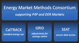 The next phase of collaboration on CalTRACK has commenced! CalTRACK and the OpenEEMeter are migrating to new governance structures and “homes” aligned with the Linux Foundation, one of the largest supporters of open source projects in the world. CalTRACK methods will continue to be developed under the umbrella of a new group called the Energy Market Methods Consortium (EM2). The CalTRACK methods working group will continue to address updates to the avoided energy use tool and two other working groups will tackle the related topics of adjustments for grid integration (GRID) and secure data transfer (SEAT). The governance of this the project and the three working groups will be under the umbrella of charters approved by the Joint Development Fund. Bruce Mast of Ardenna Energy will serving as an Interim Executive Director to administer the processes outlined in the EM2 charter. Those who would like to join a working group or the technical steering committee can contact Bruce for more information on membership. All meetings are open to the public. A video of the kick off meeting, held on February 19th, provides more detail on the structure of the EM2. Unfortunately the recording picked up the video boxes which may impair viewing of some of bullets; so the slide deck is available below the video link.
2019 Calendar For Kick Off, Working Group and Trainings in EM2 A public Google Calendar (Shared EM2 Calendar) includes all EM2 events (kick off, training, and working group meetings). You can copy specific events to your calendar or link to the public calendar. Sign up on Github to track progress on the OpenEEMeter. Thank you to all who have contributed in the past. We look forward to continued collaboration and progress in this new phase of development.
From February to July 2018 the CalTRACK working group covered four key topic areas and reported back on progress roughly each week. The list below provides quick access to the summaries by topic.
Week Twenty-Two CalTRACK Update Last week marked the final CalTRACK 2.0 working group meeting. In this meeting we discussed an update to hourly methods, an overview of our progress during CalTRACK 2.0, and suggestions for CalTRACK 3.0. You can view the final meeting at following link: Hourly Methods Update: Empirical testing has shown correlation between energy consumption and season in residential buildings, that can have an effect on the savings error. The CalTRACK 2.0 working group has proposed accounting for this seasonal effect by shortening the 12-month baseline period to 3-month weighted baseline periods. The figure below shows the effect of shortening baseline periods to 3-month on Normalized Mean Bias Error (NMBE) for residential buildings. 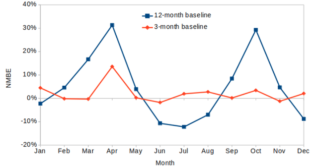 However, shortening an annual baseline to 3-month weighted baselines may not be necessary for all building types. Notably, commercial buildings tend to have a smaller seasonal effect than residential buildings, and may not experience increased NMBE from using a 12-month baseline period. The working group has established the following NMBE thresholds to define buildings that require 3-month weighted baselines and those where an annual baseline period is acceptable.
CalTRACK 2.0 Recap: Since February, the CalTRACK 2.0 process has tackled several major issues. Below is a quick synopsis of the major tasks addressed and outcomes for these topics.  Task 1: Updates to CalTRACK daily and billing methods based on feedback from CalTRACK 1.0 users. Some updates include:
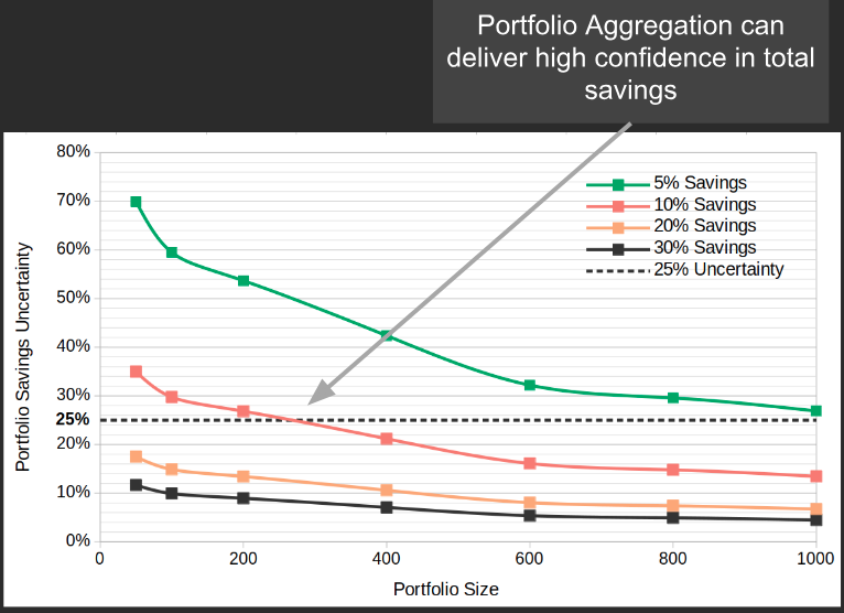 Task 2: Assess the feasibility of a portfolio aggregation approach for calculating savings as well as any effects on savings uncertainty.
Task 3: Develop a prototype method for calculating hourly savings.
Task 4: Demonstrate how price signals can adjust the value of hourly load shapes to match procurement needs.
 CalTRACK 3.0: The direction of CalTRACK 2.0 methods development was guided by feedback from use cases that required “payable savings”. For example, PG&E’s pay-for-performance energy efficiency program decided to increase compensation for energy savings during peak hours during the second iteration of their program. This required CalTRACK 2.0 to develop methods that generate savings estimates at the hourly level. Similarly, we expect CalTRACK 3.0’s tasks will be guided by the demands of stakeholders that implement programs using CalTRACK 2.0 methods. In addition, we have designed a CalTRACK 3.0 sandbox on GitHub to document issues that require further investigation. We encourage working group members to continue adding ideas to the CalTRACK 3.0 sandbox as they arise. Homework:
Week Twenty One CalTRACK Update  Energy efficiency and other distributed energy resources have the potential to bring value to the grid. The value of energy efficiency in particular has been calculated with averaged assumptions about avoided costs of producing, procuring and distributing energy from fossil fuel infrastructure, as well as other factors in some cases (e.g. avoided emissions, societal benefits etc.). This valuation is estimated at the regulatory level, when assessing the cost-effectiveness of energy efficiency, but it is usually sequestered from market actors, who have the most control over actual generated energy savings. While pay-for-performance is a key step to aligning the value of energy efficiency with the market actors responsible for it, using total annual savings as the performance metric conceals the time- and location-based value of energy efficiency which can vary significantly. This current disconnect of energy efficiency savings to its actual value to the grid or emissions avoided is an area ripe for improvements in modeling and understanding the real value of delivered energy savings. Furthermore, it is critical if energy efficiency wants to have a place at the integrated resource planning table. The availability of both hourly savings AND hourly valuations for those savings (e.g. avoided costs or emissions) allows program administrators to estimate, to a much better degree of accuracy, the value of energy efficiency to the grid. In last week’s working group discussion we covered the topic of valuation in the context of hourly load shape analysis conducted through CalTRACK 2.0. Introduction Portfolio load shapes can be used by programs that compensate for hourly energy savings and whose intention is to align the incentives with savings that are valuable to the grid when it is needed. The construction of portfolio load shapes requires:
To calculate hourly energy savings, CalTRACK methods utilize a time-of-week and temperature model. To value the energy savings, a valuation method must be applied to the hourly savings calculations. Overview of Valuation Methods There are a range of valuation strategies one can consider; which may have different effects on the outcomes. 1. Constant Valuation Energy savings are valued at a constant price across all hours of the year. 2. Step Valuation During Peak Energy savings are valued higher during peak hours of day. This valuation method assumes the peak period is the same across all days. For example, a step valuation may value energy savings from 5-8 PM 3 times more than non-peak hours of the day. 3. Avoided Cost Valuation Energy savings are valued based on their hourly avoided costs, which provides a unique value for each hour of the year. The total avoided costs include costs associated with transmission, distribution, resource portfolios, carbon and more. 4. Avoided Energy Valuation Energy savings are valued based on the cost of generating a unit of energy at the given time and location. This is similar to Avoided Cost Valuation, but only costs of generating energy are considered. Overview of Examined Scenarios Different programs and even different measures within a program will deliver different types of time-based value even if their annual savings seem similar. Here are three fairly common cases to consider for this example: 1. Home Performance Scenario Home performance improvements, which are primarily focused on weatherization and HVAC, have concentrated energy savings during periods of high and low temperatures, with little to no savings in the shoulder seasons. For example, insulated windows will generate energy savings from reduced heating during the winter and air conditioning during the summer. 2. Lighting Scenario Lighting improvements provide consistent savings year round, during hours when lighting is required. 3. Load Shifting Scenario Load shifting equipment moves energy load from high demand periods to lower demand periods. An example is an air conditioning demand response program that reduces electricity demand during peak hours. Net energy savings from load shifting programs are typically low or neutral because they cause increased energy consumption before and after the high demand period. Scenario Load Shape Analysis In the table below, the home performance, lighting, and load shifting scenarios were compared with different valuation methods. The numbers in this table represent relative value across programs (i.e. they are unit-less), making the comparison of the different methods for a particular measure/program not very meaningful. However, when each row in the table is examined separately, the type of savings that are encouraged by each valuation scheme becomes apparent. 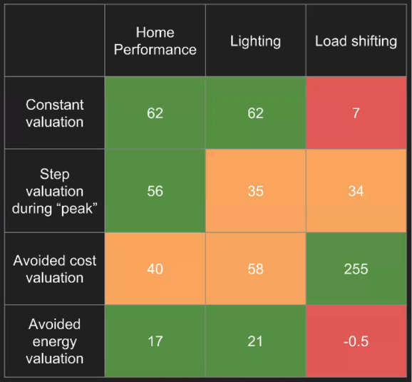 The valuation scheme will usually be a policy, market or procurement decision that should consider the ultimate outcomes intended - to ensure incentives and motivation can be aligned.
For example, if a program aims to reduce electricity grid operating costs, then an avoided cost is the most appropriate valuation method. Under this valuation method, the load shifting program is most effective. However, if a program aims to reduce net energy use, avoided energy valuation may be the most appropriate method. In this context, a market actor may decide that a lighting program is their best option. Week Twenty CalTRACK Update Over the past three weeks, CalTRACK methods testing has revolved around issues that need resolution to facilitate pay-for-performance using hourly savings. In particular, the focus has been on (i) testing and validating the Time-Of-Week and Temperature model for residential buildings and (ii) scenario analysis of different valuation methods for hourly savings. Other working group members (particularly Home Energy Analytics) contributed significant empirical results that will help in improving the robustness of the CalTRACK methods. This type of participation is the foundation for improving CalTRACK methods. Thank you for the great work! Hourly methods improvements Background: The default Time-Of-Week and Temperature model allows for extended baseline periods when fitting baseline models. When the model adaptation function is not used, a single model can be fit to the entire baseline period, which could be up to 12 months long. The single, yearly regression approach assumes that base load and weather sensitivity of energy consumption is constant throughout the year. Empirical Results: Empirical evidence shows that baseline and weather-related energy use varies during different months of the year. This variation is not represented when a single regression is estimated for the entire baseline period. Below are two potential modeling approaches:
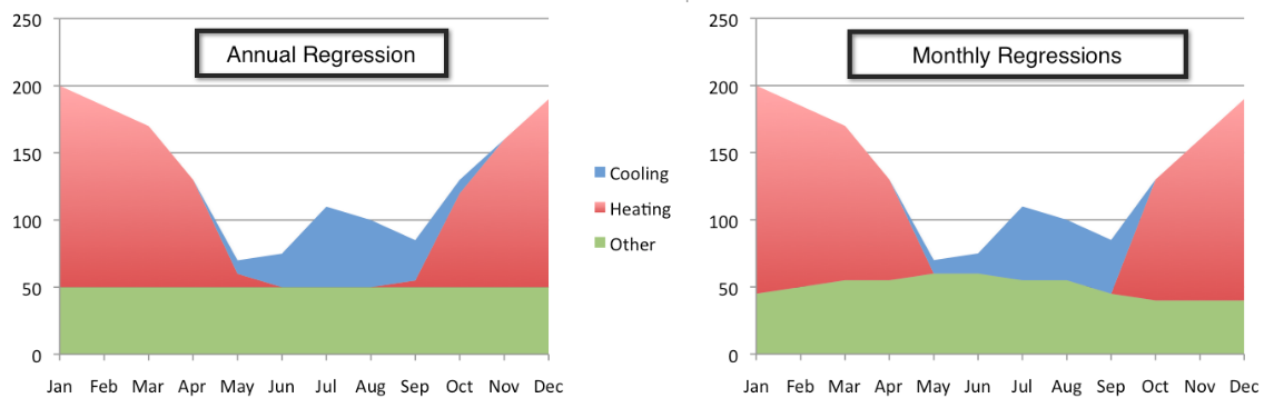 One potential problem that appears when models are fit with data from limited time periods is that without many data points, they tend to overfit the data. We can see evidence of overfitting by looking at the relationship of model error from within-sample to the model error when applied to out-of-sample data. Large discrepancies between the two values indicate potential overfitting. This relationship is evident in the figure below. 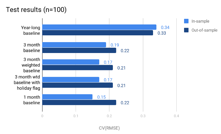 Recommendation:
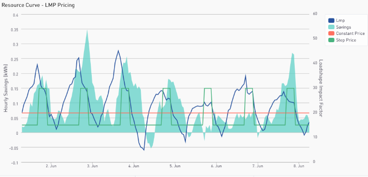
After reviewing the results of the empirical testing, we recommend applying a three-month weighted regression model for residential hourly methods. Twelve models will be fit for each month of the year, with months before and after the month of interest weighted down by 50%. For example, when predicting the counterfactual energy usage for the month of July, the corresponding baseline model will be fit using data from June, July and August of the previous year. The data points from June and August will be assigned a 50% weight compared to the data points from July. This approach accounts for varying energy consumption patterns across months of the reporting period without overfitting the model to limited data. Keep an eye out for next week’s blog post where we’ll summarize the testing of valuation methods for hourly savings. Week Eighteen CalTRACK Update Our second week of discussion on hourly portfolios included a working group meeting. You can watch the full meeting here: The value of hourly energy savings varies by use case. As such, the CalTRACK framework should be flexible to accomodate for the priorities of different use cases. A load impact factor assigns more value to energy savings during certain hours of the reporting period. For example, if a utility values energy savings 3 times more from 4-8 PM, then hourly energy savings will be multiplied by a load impact factor of three during the hours of 4-8 PM for each day of the reporting period. Each use case may need to define the load impact factors according to their desired outcomes. The portfolio-level savings are calculated by multiplying estimated hourly energy savings by the hourly load impact factor and aggregating across all hours in the reporting period. In the working group meeting we reviewed three basic methods calculating portfolio-level energy demand savings: Constant Marginal Pricing: A constant marginal pricing scheme uniformly values energy savings at each hour of the year. In this case, the load impact factor for each hour of the year is 1. This method is the simplest to compute and does not require additional data, but it fails to account for load impacts of energy savings. Static Peak Pricing: A static peak pricing scheme accounts for increased value of energy savings during peak consumption periods. A certain range of hours (ie-4-8 PM) is defined as the daily peak consumption period. The designated peak consumption period is imposed on all days of the reporting period. Static peak pricing assigns hourly load impact factors of 1 to all hours except for hours during the peak consumption period. Peak consumption period hours are given load impact factors that are greater than 1, which reflects the higher value of energy savings during these hours. Although Static Peak Pricing accounts for load impacts, its price signals are imperfect because they assume a constant peak consumption period. In reality, the peak consumption period varies throughout days of the year due to seasonality and other energy consumption trends. Real-Time Pricing: A Real-Time Pricing scheme assigns a unique load impact multiplier to each hour of the year. The load impact multipliers can be calculated according to locational marginal energy prices (LMPs). The real-time pricing scheme provides the most accurate price signals for energy savings with respect to grid impacts. The Real-Time Pricing scheme generates the most accurate price signals, but requires LMP data and there is uncertainty in hourly prices. 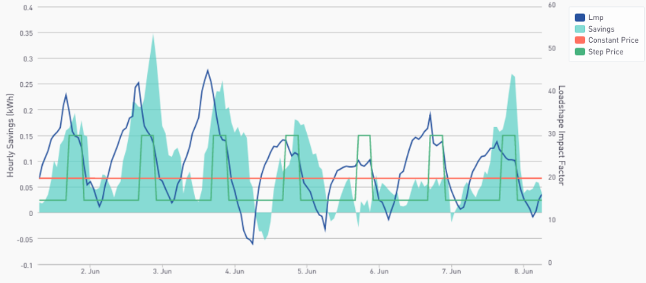 Empirical Testing:
In the coming weeks, we would like to empirically test methods for calculating portfolio-level energy savings for common use cases. Some use cases include:
Week Seventeen CalTRACK Update Establishing guidelines for aggregating building-level hourly energy savings into portfolio loadshapes requires careful consideration of information and uncertainty-level preferences for various use cases. The issues with aggregating energy savings for hourly methods and potential solutions are outlined below:  Aggregation Method for Billing Period and Daily Methods: In daily and billing period methods, building-level savings are generated by summing the building’s estimated energy savings for each day or billing period of the reporting period. The portfolio savings are then calculated by aggregating total savings for each building in the portfolio. Why are daily and billing period aggregation methods problematic with hourly models? For hourly models, portfolio uncertainty is difficult to calculate when savings are aggregated for each hour due to correlation in the error term. Suggested Hourly Aggregation Methods: To begin our discussion of hourly aggregation methods, consider two types of roll-ups: Vertical Roll-Ups: In a vertical roll-up, hours within a day are grouped together for each building before aggregation. For example, one may choose to aggregate hourly energy savings in three-hour intervals throughout the day instead of each hour individually. Although vertical roll-ups can reduce portfolio uncertainty, larger time intervals provide less information in portfolio loadshapes. Hourly methods are created to provide granular information about energy load impacts during each time-of-day. Less information is available if hours are “rolled-up” into larger time intervals. Horizontal Roll-Ups: Horizontal roll-ups aggregate each hourly estimate with estimates of the same hour across weeks. A horizontal roll-up can aggregate individual hours or time intervals, such as the three-hour interval discussed above. 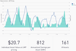 Other Considerations: There were a few additional suggestions from the working meeting (5/24) that could help create guidelines for aggregating portfolio loadshapes:
Homework:
Week Sixteen CalTRACK Update  During the standing meeting on 5/24, the working group finalized hourly methods for calculating hourly energy savings and commenced discussion on aggregating hourly savings into portfolio loadshapes. The finalized hourly methods and an introduction on aggregating portfolio loadshapes are outlined below. Finalized Hourly Methods:
Aggregating Hourly Savings into Portfolio Loadshapes
To provide an accurate valuation of energy efficiency as a grid resource, energy savings must be quantified at specified time intervals and geographic locations. To create portfolio loadshapes, building-level savings must be aggregated. The method of aggregation has implications on the portfolio uncertainty and provides different granularity of information for aggregators, utilities, and customers. Different use cases may prefer different aggregation methods based on priorities specific to their use case. To accommodate different use cases, flexible methods for aggregating hourly savings into portfolio loadshapes may be preferred. As we explore this topic further, some potential use cases to consider are: Pay-for-Performance Programs In the PG&E pay-for-performance program, the utility provides incentives for peak savings. This requires estimates of portfolio savings at the hourly level. Non-Wires-Alternative Procurement Non-Wireless-Alternative procurements require estimates of portfolio savings for buildings connected to specific grid nodes in order to measure grid impacts and potentially avoid infrastructure investments. Cap and Trade, Greenhouse Gases, or Carbon Tracking or Trading Initiatives Initiatives attempting to accurately quantify carbon offsets from energy efficiency investments require savings estimates at specified time and geographic locations because generation portfolios utilize resources with different carbon intensity at different times and locations. We discussed a few options for aggregation methods, and look forward to input from the working group in the coming week. Week Fourteen & Fifteen CalTRACK Update Review of hourly method proposals continued in week fourteen of CalTRACK 2.0 and will be finalized at the 5/24 working group meeting. Lawrence Berkeley National Lab’s Time-of-Week Temperature (TOWT) model is the specification to be used in CalTRACK 2.0. Mathieu et al. describe the application of TOWT models in Quantifying Changes in Building Electricity Use, with Application to Demand Response. Overview of TOWT models: As energy efficiency finds its legs as a grid resource, time dependent savings will be essential to the value proposition. Pay-for-performance programs can leverage this value with accurate building-level energy savings calculations at granular time intervals. TOWT models are one method for calculating energy savings at the hourly level. Strengths:
 Weaknesses:
|
The purpose of this blog is to provide a high-level overview of CalTrack progress.
For a deeper understanding or to provide input on technical aspects of CalTrack, refer to the GitHub issues page (https://github.com/CalTRACK-2/caltrack/issues). Recordings
2019 CalTRACK Kick Off:
CalTRACK 2.0 July 19, 2018 June 28, 2018 June 7, 2018 May 24, 2018 May 3, 2018 April 12, 2018 March 29, 2018 March 15, 2018 March 1, 2018 February 15, 2018 February 1, 2018 Archives
March 2024
|
||||||
 RSS Feed
