
|
Week Thirteen Update for CalTRACK  During week thirteen, the CalTRACK working group discussed proposals for hourly methods in the standing meeting. The discussions included helpful suggestions of other reference materials as well as variations that may be appropriate for different applications of hourly methods and suggested improvements in CalTRACK 2.0’s documentation. The video from May 3, 2018 is provided at the end of this post. Hourly Methods In the development of hourly methods, the goal is to establish guidelines that mirror the methodology in billing period and daily methods. However, hourly methods have unique complexities that require departures from billing period and daily methods. These complexities are identified and discussed below: Data Management When compared to hourly data, daily and billing period savings calculations have higher data sufficiency requirements because hourly data contains more information per time period. This characteristic of hourly data supports the two adjustments to hourly data sufficiency requirements listed below: 1. Usage data sufficiency will be specified in terms of data coverage (or common support) instead of a minimum time period: Daily and billing period data sufficiency requirements impose a minimum quantity of time observed from a year of data. In hourly methods, usage data sufficiency will be specified in terms of data coverage in the independent variables. In Time of Week and Temperature (TOWT) models, the independent variables are temperature and occupancy. Data sufficiency requirements will be based on LBNL recommendations for data coverage. 2. Missing Data Temperature has less variation between hours than days or billing periods. Smaller temperature variation between hours increases the likelihood that interpolated temperature values are accurate. For this reason, interpolated temperature values will be allowed in the reporting period for hourly methods. The threshold of allowable interpolated hours will be determined through empirical testing. Recommendation for Pay-for-Performance Use Case:
Time Of Week Temperature (TOWT) Modeling Approach The TOWT model, originally by Lawrence Berkeley Lab, contains two covariates: Occupancy: Occupancy is an indicator variable that takes the value of 1 if the building is occupied in the hour and 0 otherwise. In LBNL’s model, occupancy of a building is defined by:
The TOWT model allows user-defined temperature bins for modeling a building’s weather dependence. We are recommending setting 7 fixed bins with endpoints at 30, 45, 55, 65, 75, 90, in order to cover a wide variety of climate conditions. Use Case and Uncertainty Time-aggregated Uncertainty: In the program evaluation use case, an analyst may be interested in obtaining time-aggregated savings and uncertainty. Due to residual autocorrelation at the hourly level, aggregating hourly uncertainty for larger time intervals creates imprecise standard errors and uncertainty calculations. Instead, we recommend using daily methods with improved ASHRAE or Ordinary Least Squares (OLS) formulations of Fractional Savings Uncertainty (see Koran 2017) for aggregating uncertainty over time periods. Hour-level Uncertainty Estimates: For the procurement and pay-for-performance use cases, regression analysis is an effective tool for acquiring point estimates of savings and uncertainty at each hour. If each building is assumed to have independent errors, the uncertainty at each hour for all buildings in the portfolio can be aggregated without an autocorrelation problem. Methods Documentation Currently, the documentation for CalTRACK 2.0 is being updated. The first half of CalTRACK 2.0’s documentation will be posted on GitHub to allow the working group to review and comment on the changes in documentation. Similar to the methods, the development of effective documentation is an iterative process. The documentation for CalTRACK 2.0 will improve by dividing into three distinct documents: 1. Methods This document outlines the methodology for quantifying billing period, daily, and hourly energy savings while maintaining CalTRACK-compliancy. In CalTRACK 2.0, the Methods will be organized with a numbering system that corresponds to the Methodological Appendix. This will make referencing and accessing the appendix easier. 2. Methodological Appendix The Methodological Appendix summarizes discussions and empirical testing that justify methodological decisions. The Methods will reference sections in the Methodological Appendix for readers to easily access empirical support for methodological decisions. 3. Field Guide A document with minimum requirements for an implementation to maintain CalTRACK-compliancy. This is designed to be a practical and accessible checklist for analysts and other implementers of CalTRACK. Ideas for Future CalTRACK Work A sandbox has been added to the GitHub site to document proposals for participants to add ideas for future CalTRACK iterations. If you have an idea for CalTRACK 3.0, or beyond that cannot be addressed this year, please add it the the sandbox. Additional Hourly Methods Resources
Homework
0 Comments
Week Twelve CalTRACK Update During week twelve, we continued our discussion of hourly methods. In the upcoming week, we will analyze test results for hourly methods on GitHub. We will also be talking about how to log ideas for future improvements. The standing meeting to discuss hourly methods will be on Thursday, May 3rd at 12:00 (PST).  Homework:
Week Eleven CalTRACK Update Week eleven was the first week of hourly methods discussion. Developing hourly methods will require discussion and empirical testing of topics unique to hourly methods before we can make final specifications. Topics that must be addressed include:
Time Of Week Temperature Models (TOWT): A proposed model for hourly methods is the TOWT model from Lawrence Berkeley National Labs (LBNL) is shown below. 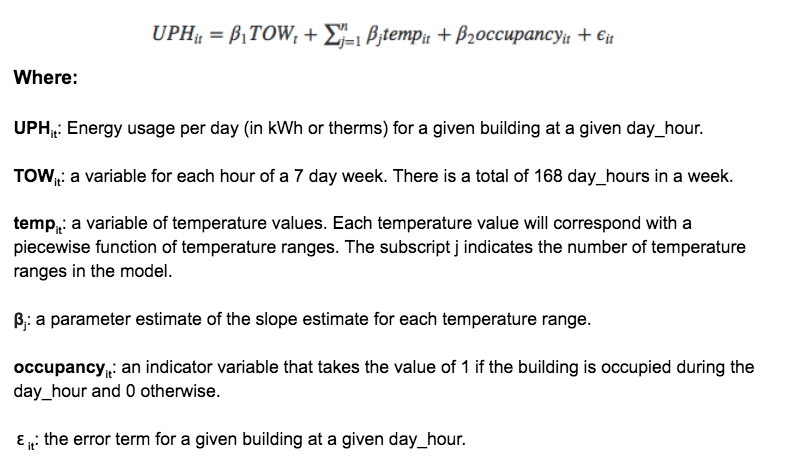 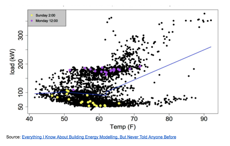 Notes:
Homework:
Week Ten CalTRACK Update The CalTRACK working group finalized discussions on Building Qualifications during the first half of Thursday’s (4/12) meeting and dove into the hourly methods during the second half. Bill Koran from SBW consulting provided a helpful overview of hourly models and the ECAM energy data analysis tool. The major findings of this meeting are summarized below: Building Qualification Observations and Recommendations: Main observations that were driving the recommendations:
 Goals for Hourly Methods: Hourly models are necessary for estimating the load impact of energy efficiency. This makes hourly energy savings important information for aggregators and utilities in an energy efficiency marketplace. Our goal is to establish suitable methods for calculating whole building hourly energy savings for residential and commercial buildings. Additionally, the methods will include guidelines for aggregating site-level savings. Discussion Topics: We have allotted three weeks to test and discuss hourly methods. Below are some important topics that will need to be addressed:
Homework:
Week Nine CalTRACK Update During week nine of CalTRACK, there were continued discussions on building qualification criteria and some introductory comments on hourly methods. The working group meeting will be held on Thursday, April 12th at 12:00 (PST). We will discuss:
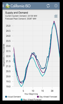
Hourly Methods Overview: Hourly methods are a new addition in CalTRACK 2.0 and were not in the first version of CalTRACK. This task involves testing various hourly modeling methods and recommending a standardized approach to hourly modeling, which can reveal the time value of energy efficiency. Importance of Hourly Methods:
 Time Of Week and Temperature Models: To start the discussion of hourly methods, it is helpful to consider to existing open source tools. Lawrence Berkeley National Lab has developed an open source time of the week and temperature (TOWT) model to calculate hourly energy savings and is part of the RMV2.0 - LBNL M&V2.0 Tool. A TOWT model predicts hourly energy savings by utilizing hourly temperature data instead of daily or billing period HDD and CDD. Another is ECAM (ENERGY CHARTING & METRICS) developed by Bill Koran at SBW consulting. We look forward to discussion on the working group call about these approaches, and more to frame the approach to empirical tests for the CalTRACK 2.0 hourly methods. Final Note: It is important to remember that CalTRACK methods development is an iterative process. The finalized methods for CalTRACK 2.0, just like v. 1.0, will benefit from field deployment and may need to be revised in future years. We expect this process to result in improved and refined methods with successive iterations. Homework:
Building Qualifications Test Reveals Wide Applicability of CalTRACK Method for Portfolio Analysis3/29/2018 Week Eight CalTRACK Update Today we had an exciting working group meeting focused on Building Qualifications with test results and recommendations. We will be stepping into hourly methods in the upcoming week. Daily and Billing Period Methods Specifications: The final comments on daily and billing period methods have been received. The new, finalized specifications are currently being updated you can track the final on GitHub Issue #82. Participants can review the final specifications and track any issues that fed into the final specification prior to their publication at this site. Building Qualifications: The CalTRACK methods are equipped to normalize for weather’s effect on a building’s energy consumption. The methods become unreliable when a building’s energy consumption patterns are instead correlated with non-weather variables. For example, irrigation pumps are used on an agricultural cycle rather than in response to temperature changes. It is reasonable to expect higher energy consumption during the growing season and an analyst may suggest re-specifying the model to control for these seasonal variations. Without modification, existing billing and daily CalTRACK models cannot accommodate these nuanced cases. For this reason, buildings that are not well-specified by the CalTRACK model should be identified and removed from portfolios because they have significant effects on portfolio uncertainty. This issue can be tracked on GitHub Issue #71. 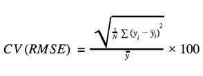 Building Qualification Metric: To evaluate a building’s qualification status, a metric and a thresholds should be defined. After empirical testing, the recommended metric for CalTRACK 2.0 is CV(RMSE). Justification:
Building Type: Building type can be a useful identifier for aggregators to determine a building’s suitability for a portfolio. In figure 1, the relationship between energy consumption and CV(RMSE) is measured by building type. The size of each dot corresponds with the number of meters per building type. 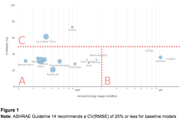 The CalTRACK methods will be most effective for buildings in region A, which have relatively low energy consumption and low CV(RMSE). Buildings in region B are high energy consumers. These buildings often have a single meter tracking consumption for various sub-buildings with mixed uses, which make it difficult to quantify the effect of an energy-efficiency intervention on overall consumption. These buildings will likely require custom M&V and not qualify for CalTRACK. The buildings in region C have high CV(RMSE). The high CV(RMSE) is likely due to correlation in energy usage that is not specified in the model, such as seasonality. These models should not qualify for CalTRACK. CV(RMSE) Threshold for Building Qualification: Due to differences in model quality, portfolio size, and building type between aggregator datasets, it is difficult to establish a universally applicable building-level CV(RMSE) cut-off. The graphs below visualize the relationship between building-level CV(RMSE), portfolio uncertainty, and building attrition. The various graphs show these relationships with different building types and portfolio sizes. While analyzing the graphs, consider that procurers and aggregators tend to be more concerned with portfolio-level uncertainty and building attrition than the building-level CV(RMSE), especially for pay-for-performance programs and Non-Wires Alternatives procurements. 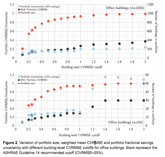 The results show that strict building-level thresholds of 25% CV(RMSE) result in low portfolio uncertainty, but significant building attrition. Also, the results vary depending on the portfolio size and building type. From an aggregators perspective, it may be preferable to adopt a less restrictive building-level CV(RMSE) threshold and focus on minimizing building attrition with respect to a strict portfolio uncertainty threshold. Recommendations: We are recommending that the specific building eligibility requirements be generally left to the procurer, who can set the requirements that align best with their goals for a procurement, provided these are specified clearly upfront. CalTRACK can provide general guidelines as follows.
Other Reading Cited in the Working Group Meeting today: Normalized Metered Energy Consumption Draft Guidance CPUC ASHRAE Guideline 14 Homework:
Week Seven CalTRACK Update A quick update for this week and a reminder of the working group meeting: Thursday, March 29th at 12:00 (PST) in which we will cover:
 During week seven of CalTRACK, consideration of building qualification methods continued. This week’s working group meeting will conclude the discussion of building qualification methods and launch the testing period. Comments or test results should be added on GitHub issues early next week to ensure they can be considered before proposals are finalized.
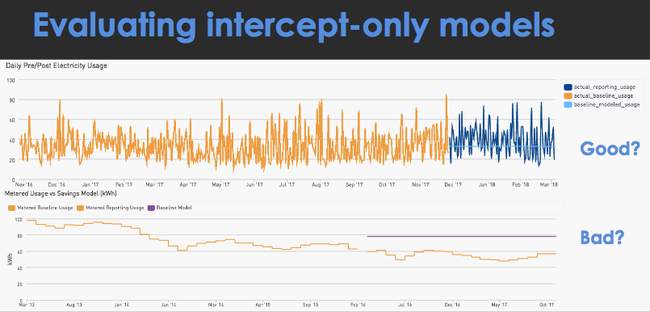
Homework: Week Six CalTRACK Update Week six was primarily focused on the building qualification discussions and will continue to be the focus of testing and experimentation this week; this was coming off of an exciting working group meeting on March 15, 2018 linked below. 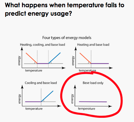 Review of properties of intercept-only models in PRISM: As we analyze building qualifications, it is useful to review the properties of PRISM intercept-only models to ensure they are properly treated. Here are a few characteristics of intercept-only models: Properties:
 Description of Each Proposed Metric: During the upcoming week, we will use empirical testing to establish the preferred metric and threshold to determine a building’s suitability for CalTrack methods. The two proposed metrics are described below: 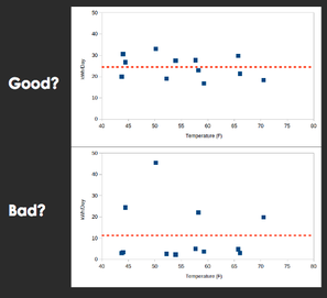 Coefficient of Variation Root-Mean-Square-Error (CVRMSE) The CVRMSE is calculated by:
Mean Absolute Percent Error (MAPE) The MAPE is calculated by:
Other Reference Materials on Baseline Models that inform the discussion: In the Granderson, et. al. study cited below, one key question it tackled was: “How can buildings be pre-screened to identify those that are highly model predictable and those that are not, in order to identify estimates of building energy savings that have small errors/uncertainty?”
Suggestions on Testing These Metrics Remember, our goal for testing is to establish our preferred metric and threshold for building qualification. When testing the CVRMSE and MAPE metrics, we have some suggestions to yield the most informative results:
Non-Routine Adjustments: Some discussion arose regarding the possibility of making non-routine adjustments for sites that are outliers. CalTRACK 1.0 addressed this issue by stipulating specific criteria for accepting a non-routine adjustment. Specifically, if savings exceeded 50% +/-, either party would be able to make an appeal to remove the project from the portfolio. Other specific considerations may be related to program eligibility, such as a house that adds solar panels during a performance period. At a general level, CalTRACK methods shy away from stipulating methods for non-routine adjustments, as these tend to demand substantial additional effort and may require additional data that would run contrary to the premise of using CalTRACK methods in the first place. As CalTRACK 1.0 testing demonstrated, for aggregators of residential projects, larger sample sizes diminish the effect of these outliers. Participant Homework:
Week Five CalTRACK Update We look forward to another working group meeting Thursday March 15th. Here are some updates from the activity last week. Building Qualification Summary: During the past week, we started discussions to establish an empirical method to determine a building’s suitability for CalTRACK methods. Listed below are two topics related to building qualifications that require testing:
Homework for Participants:
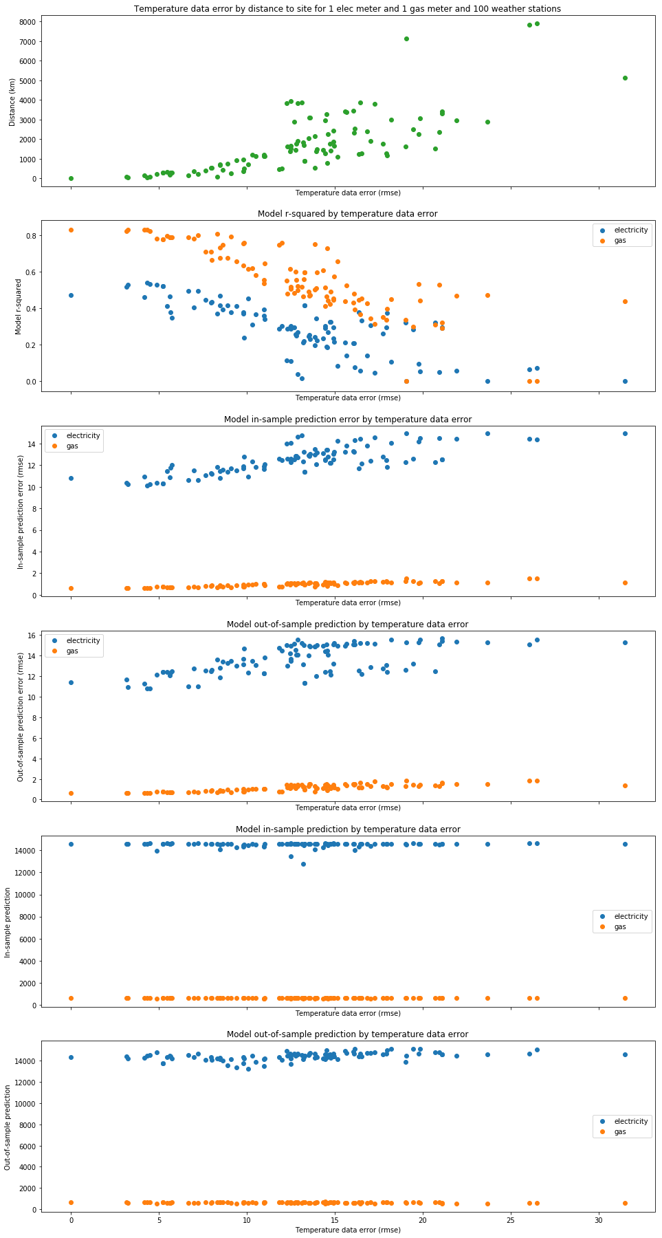
 Week Four CalTRACK Update During week 4, we received some interesting results from tests on daily and billing period methods. In this week’s blog post, we analyze the test results and determine their effect on our proposed daily and billing period methods. Additionally, we will introduce the new topic of building qualifications. (Participant Homework can be found at the bottom of this post) Test Results: 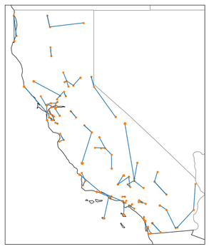 Weather Station Mapping: Because we do not have access to weather data at the location of each site, the best approach for estimating a site’s temperature is to use data from nearby, high-quality weather stations. The most intuitive way to “map” which primary and backup weather stations to use for a site is to simply choose weather stations with the shortest distance to the site. Some argue that this simple method fails to account for the unequal distribution of weather patterns over space. For example, imagine a mountain home is technically closer to a weather station in the desert valley than to another weather station in the mountains. We might expect the house’s weather data to be better approximated by the mountain weather station than the desert valley weather station, despite it being further away. To account for this phenomenon, another proposal is to use pre-defined climate zones throughout states to choose the closest primary and backup weather stations that are within that site’s climate zone. Two proposals for mapping a site’s weather stations:
To empirically inform our decision, we ran a simulation for each mapping method where we used the actual weather stations as units, instead of the sites, and compared each method’s accuracy. Our results show that both proposed methods provide very similar results, with “Method 1” and “Method 2” providing a perfect match 53% and 56% of total matches respectively. These results indicate that there are not significant accuracy reductions from choosing the simpler “Method 1".
Results:
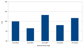 Maximum Baseline Period Length: There have been discussions about defining a maximum baseline period because excessively long baseline periods may absorb unnecessary variation that could obscure our model predictions. To determine the effect of longer baseline periods, we calculated baselines of 12, 15, 18, 21, and 24 months. The graph below shows that normalized annual consumption (NAC) can be unstable as we increase the baseline period. Recommendation:
Degree Day Balance Points: A proposed new method for CalTRACK 2.0 is to use variable balance points instead of fixed balance points on the HDD and CDD variables. In the figure below, we can see that buildings tend to cluster at the limits of balance point degree ranges, which implies that some results may be constrained by small search grids. When the degree range is expanded, the results displays a distribution that is closer to Gaussian. 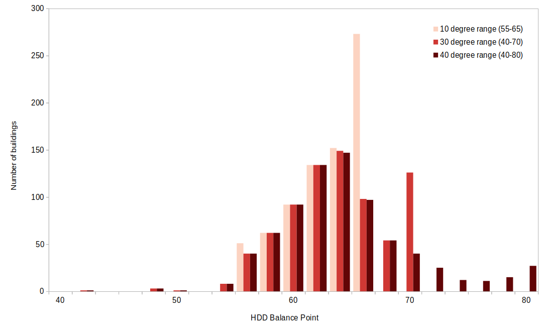 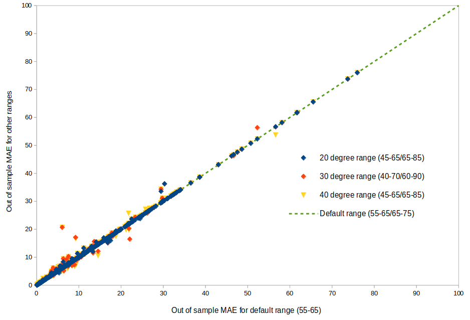 Although expanding the search grid may uncover a balance point that yields a higher R-squared, the figure on the right shows that these results have a nominal impact on model fit. Regardless, variable balance points are advised because they provide better balance point estimates, which have more interpretation value. Recommended Allowable Ranges: HDD: 40-80 CDD: 50-90
In CalTRACK 2.0, we intend to eliminate the p-value screen and select models strictly on the adjusted R squared. We suggest this change because the p-value screen does not increase our model fit and we lose valuable information on estimators when we drop them due to high p-values, as well as eliminating many weather-sensitive model fits. Handling Billing Data: Modeling using billing data was underspecified in CalTRACK 1.0. We are proposing to include explicit instructions on modeling using billing data that includes billing periods of different lengths using weighted least squares regression. New Topics: Building Qualification: In this coming week, we will begin our examination of building qualification screening criteria. The CalTRACK methods were initially tested using residential buildings and are currently mainly used to quantify energy savings for residential units and small commercial buildings. The limits of the CalTRACK methods for measuring savings in commercial or industrial buildings (where weather is likely to be a poorer predictor of energy consumption) has been subject to less scrutiny. Our goal is to create empirical tests for determining the energy usage patterns in buildings that qualify a building for CalTRACK methods and exclude those that would be better estimated with different methods. We are looking forward to your input on potential methods and tests to define buildings that qualify for CalTRACK. Some questions that need to be addressed (and we welcome additional questions):
We are looking forward to your input on building qualification in this coming week. There will be a lot to discuss on GitHub Issues. We would like to test proposed building qualification methods empirically before making decisions, so it is important to make method and testing suggestions as soon as possible. HOMEWORK:
|
The purpose of this blog is to provide a high-level overview of CalTrack progress.
For a deeper understanding or to provide input on technical aspects of CalTrack, refer to the GitHub issues page (https://github.com/CalTRACK-2/caltrack/issues). Recordings
2019 CalTRACK Kick Off:
CalTRACK 2.0 July 19, 2018 June 28, 2018 June 7, 2018 May 24, 2018 May 3, 2018 April 12, 2018 March 29, 2018 March 15, 2018 March 1, 2018 February 15, 2018 February 1, 2018 Archives
March 2024
|

 RSS Feed
